The data preparation for any analysis begins with data screening and tests of assumptions. The data screening ensures the data are correct and the tests of assumptions ensure the data are suited for the type of analysis to be conducted. The Module 6 assignment is to conduct data screening for a regression analysis, and then in Module 7, you will conduct the regression analysis. In fact, you will need to conduct the analysis as part of the tests of assumptions, so I encourage you to do both assignments at the same time.
This post will guide you through the data screening for a regression analysis. It is important to note these procedures are the same for multiple regression, moderator analysis, and mediator analysis, as all are types of multiple regression.

As a reminder, a multiple regression tests the extent to which two or more predictor variables (Xi) account for the variance in an outcome variable, more formally known as the criterion variable (Y).
Multiple regression
Regression assesses the following hypothesis:
RQ: To what extent, if any, do Neuroticism and Stress account for the variance in Depression?
H0: Neuroticism and Stress do not significantly account for the variance in Depression.
H1: Neuroticism and Stress significantly account for the variance in Depression.
Based upon the research question and hypotheses, the variables for this assignment are the predictor variables (X) Neuroticism, as measured by IPIP-Neuroticism, and Stress, as measured by DASS-Stress. Both are continuous variables with interval levels of measurement. The criterion variable (Y) is Depression, as measured by DASS-Depression, a continuous variable with interval level of measurement.
To guide us through the data screening and testing of assumptions, which I will show concurrently, I will use the following assumptions (Laerd, 2021):
- There must be one criterion/outcome variable that is measured at the continuous level (i.e., the interval or ratio level).
- There must be two or more predictor variables that are measured either at the continuous or nominal level.
- There must be independence of observations (i.e., independence of residuals).
- There must be a linear relationship between (a) the criterion/outcome and each of the predictor variables, and (b) the criterion and predictor variables collectively.
- There must be homoscedasticity of residuals (equal error variances).
- There must be no multicollinearity.
- There must be no significant outliers, high leverage points, or highly influential points.
- The residuals (errors) must be approximately normally distributed.
Data Screening: Frequency tables
Frequency tables are used to see the approximate distribution of the variables. The frequency tables will show you an approximate distribution of the variables Neuroticism, Stress, and Depression.
With the frequency tables completed, the remaining data screening tasks (i.e., tests for outliers, tests of linearity, tests of normality) are included within the tests of assumptions.
- There must be one criterion/outcome variable that is measured at the continuous level (i.e., the interval or ratio level). The criterion variable, Depression, is continuous (interval level of measurement) by research design.
- There must be two or more predictor variables that are measured either at the continuous or nominal level. The predictor variables are Neuroticism and Stress, both of which are continuous (interval level of measurement) by research design.
- There must be independence of observations (i.e., independence of residuals). Independence of observations (autocorrelation) is tested using the Durbin-Watson statistic. The Durbin-Watson statistic is developed when one conducts the regression as part of the output. Values of the Durbin-Watson statistic close to 2 indicate no autocorrelation (independence of observations). Values of 1 to 3 satisfy this requirement.
- There must be a linear relationship between (a) the criterion/outcome and each of the predictor variables, and (b) the criterion and predictor variables collectively. The linear relationship between variables may be tested by scatterplot for each pairing with the criterion, as well as by an examination of the plot of the residuals. This is a visual test.
- There must be homoscedasticity of residuals (equal error variances). The assumption is tested using a visual test. One examines the plot of residual (error) variances to determine if the residuals are relatively equal as indicated by a box shape across the figure. Instances in which the residuals are cone-shaped indicate a lack of homoscedasticity.
- There must be no multicollinearity. Tested using the variance inflation factor (VIF), a score of 4 or less indicates no multicollinearity. Multicollinearity is the phenomenon when the predictor variables approximately measure the same construct. If multicollinearity is present, it may be eliminated by removing one of the variables from the analysis.
- There must be no significant outliers, high leverage points, or highly influential points. The assumption is tested using casewise diagnostics, which identify these three phenomena. Instances of these points should be removed from the dataset and the dataset reevaluated. If SPSS does not report any results for casewise diagnostics, it means that no multivariate outliers, high leverage points, or highly influential points are present and the assumption has been met. If SPSS does not produce any output for casewise diagnostics, there are no significant outliers, high leverage points, or highly influential points to consider.
- The residuals (errors) must be approximately normally distributed. The test of residual normality is tested using a P-P plot.
Mediation analysis
The test for mediation analysis is the same as for multiple regression above. The research question and hypotheses will be different, as shown. In this example, the predictor is Stress (X), the mediator is Neuroticism (M), and the criterion is Depression (Y).
RQ: To what extent, if any, does Neuroticism mediate the predictive relationship between Stress and Depression?
H0: Neuroticism does not significantly mediate the predictive relationship between Stress and Depression.
H1: Neuroticism significantly mediates the predictive relationship between Stress and Depression.
Moderator analysis
The tests of assumptions for moderator analysis is identical as for multiple regression above. The significant difference for the example provided by the following research question and hypotheses is one of the variables, the moderator of gender (W) is categorical (nominal level of measurement). This change still meets the tests of assumptions. The predictor is Stress (X) and the criterion is Depression (Y). A moderator variable is a type of predictor variable. Therefore, when conducting tests of assumptions, include the moderator (W) as a predictor (X).
RQ: To what extent, if any, does gender moderate the predictive relationship between Stress and Depression?
H0: Gender does not significantly moderate the predictive relationship between Stress and Depression.
H1: Gender significantly moderates the predictive relationship between Stress and Depression.
Conducting the tests of assumptions for multiple regression (video – 10 min)
Writing up the assignment
Review the assignment instructions. You are to identify the three variables you will use in the assignment. These variables must come from the dataset in Week 2 Data Screening Assignment as you described in the Week 2 Quiz: Pick Topic assignment. If you are completing a mediation analysis, you may consider selecting an additional continuous variable, just as I have done in the example above in which I added Stress. Mediation may be done with a categorical mediator; however, interpreting the results is easier (and easier for learning) if a continuous variable is used. For this example and in anticipation of completing a moderator analysis (Example 3), the variables are stated below.
Predictor variable (X): Stress, as measured by DASS-Stress, a continuous-interval level of measurement variable.
Moderator variable (W): Gender, as self-reported, a categorical-nominal level of measurement with classes of male and female.
Criterion variable (Y): Depression, as measured by DASS-Depression, a continuous-interval level of measurement variable.
Writing up the narrative should begin with an introduction.
Data screening was accomplished for the variables of gender, Stress, and Depression from the EDCO 745 course dataset to test the null hypothesis that gender does not significantly moderate the predictive relationship between Stress and Depression.
The next sentences will describe the data screening and tests of assumptions and any notable results from each.
A frequency table was created for gender (see Table 1). Results of the frequency table indicated slightly more male (n = 704) than female (n = 596) participants (Table 1).
Table 1
Frequency for Gender
| Frequency | Percent | Valid Percent | Cumulative Percent | ||
| Valid | Male | 704 | 54.1 | 54.2 | 54.2 |
| Female | 596 | 45.8 | 45.8 | 100.0 | |
| Total | 1300 | 99.9 | 100.0 | ||
| Missing | 2 | .1 | |||
| Total | 1302 | 100.0 | |||
Tests of assumptions were completed for multiple regression.
- There must be one criterion/outcome variable (Y) that is measured at the continuous level (i.e., the interval or ratio level). The criterion variable, Depression, is continuous (interval level of measurement) by research design.
- There must be two or more predictor variables (Xi) that are measured either at the continuous or nominal level. The predictor variables are gender and Stress. Gender, the moderator variable (W), which is a type of predictor, is a nominal level of measurement and Stress is continuous (interval level of measurement) by research design.
- There must be independence of observations (i.e., independence of residuals). Independence of observations (autocorrelation) is tested using the Durbin-Watson statistic. The Durbin-Watson statistic is developed when one conducts the regression as part of the output. Values of the Durbin-Watson statistic close to 2 indicate no autocorrelation (independence of observations). Values of 1 to 3 satisfy this requirement. The Durbin-Watson statistic for the regression is 2.076, demonstrating independence of observations (see Table 2).
Table 2
Model Summary

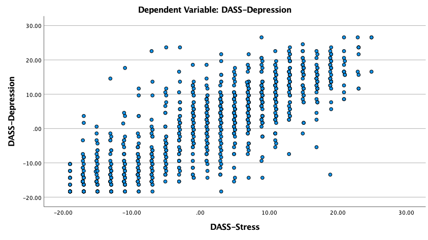
- There must be a linear relationship between (a) the criterion/outcome and each of the predictor variables, and (b) the criterion and predictor variables collectively. The linear relationship between variables may be tested by scatterplot for each pairing with the criterion, as well as by an examination of the plot of the residuals. This is a visual test. Based upon a scatterplot between Stress and Depression, there is a linear relationship between the two variables (see Figure 1).
Figure 1
Scatterplot of Stress and Depression

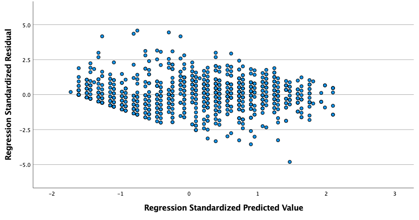
Because gender is a nominal variable, a scatterplot cannot be developed for relationships with this variable. However, one may examine the overall linearity of the model, which is the combination of gender and Stress in relation to Depression, which is completed through partial regression plots. Based upon the result of the partial regression plot, there is a linear relationship (See Figure 2).
Figure 2
Partial Regression Plot of Predictors Gender and Stress Against Depression

- There must be homoscedasticity of residuals (equal error variances). The assumption is tested using a visual test. One examines the plot of residual (error) variances (Figure 2) to determine if the residuals are relatively equal as indicated by a box shape across the figure. Instances in which the residuals are cone-shaped indicate a lack of homoscedasticity. Figure 2 indicates a slightly diamond shape with narrowing at each end, indicating homoscedasticity of residuals is questionable.
- There must be no multicollinearity. Tested using the variance inflation factor (VIF), a score of 4 or less indicates no multicollinearity. Multicollinearity is the phenomenon when the predictor variables approximately measure the same construct. If multicollinearity is present, it may be eliminated by removing one of the variables from the analysis. The VIF for the present analysis is 1.007, indicating no multicollinearity, and is presented in Table 3 in the far-right column.
Table 3
Regression Coefficients

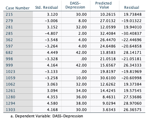
- There must be no significant outliers, high leverage points, or highly influential points. The assumption is tested using casewise diagnostics, which identify these three phenomena. Instances of these points should be removed from the dataset and the dataset reevaluated. Casewise diagnostics were completed for the regression, revealing 16 records with extreme violations, as shown in Table 4. These records will be removed prior to completing the regression.
Table 4
Casewise Diagnostics

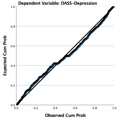
- The residuals (errors) must be approximately normally distributed. The test of residual normality is tested using a normal P-P plot. Normality is indicated when the points of the scatterplot fall along or near the 45-degree line. The normal P-P plot for the regression indicates an approximately normal distribution of the residuals. See Figure 3.
Figure 3
Normal P-P Plot of Regression Standardized Residuals

Note that within the write up, each line references the table or figure that supports the statement being made. This also requires one to correctly label each of the tables or figures prior to submitting the assignment. Also, please note in the sample write-up that the tables are correctly formatted according to APA and they are not directly copied from SPSS, which are not in APA format.

Submitting the assignment
When submitting this assignment, you must first describe the data screening assignment. The write-up should be descriptive of the variables and the activities used to screen the data, along with a description of the results. All submissions must be a single Microsoft Word document. Do not submit the SPSS file.

